Today, in my Statistics and Probability course, I arrived to the lecture an hour early for some reason… So I had an hour of just looking into the air in this large auditorium. What do I do? Well, I could read ahead or do some assignments. Or—because it was a statistics course after all—I could do some statistics! So I decided to record the arrival times of every person to this lecture and analyze its distribution. What will we find? Probably nothing much. A lot of real-life things don’t follow any particular well-known distribution. But now I’m here, so I might as well.
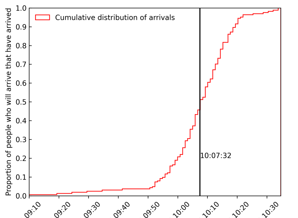
What I found was initially slightly surprising to me, because I didn’t expect to find anything but I did find something. Some fun facts are that the mean arrival time was 10:07:32 on this particular day, with the lecture beginning at 10:15, and that 10.4% (17 out of 164) of attendees arrived more than five minutes late.
In the cumulative distribution plot below, you can see the arrival times visualized.

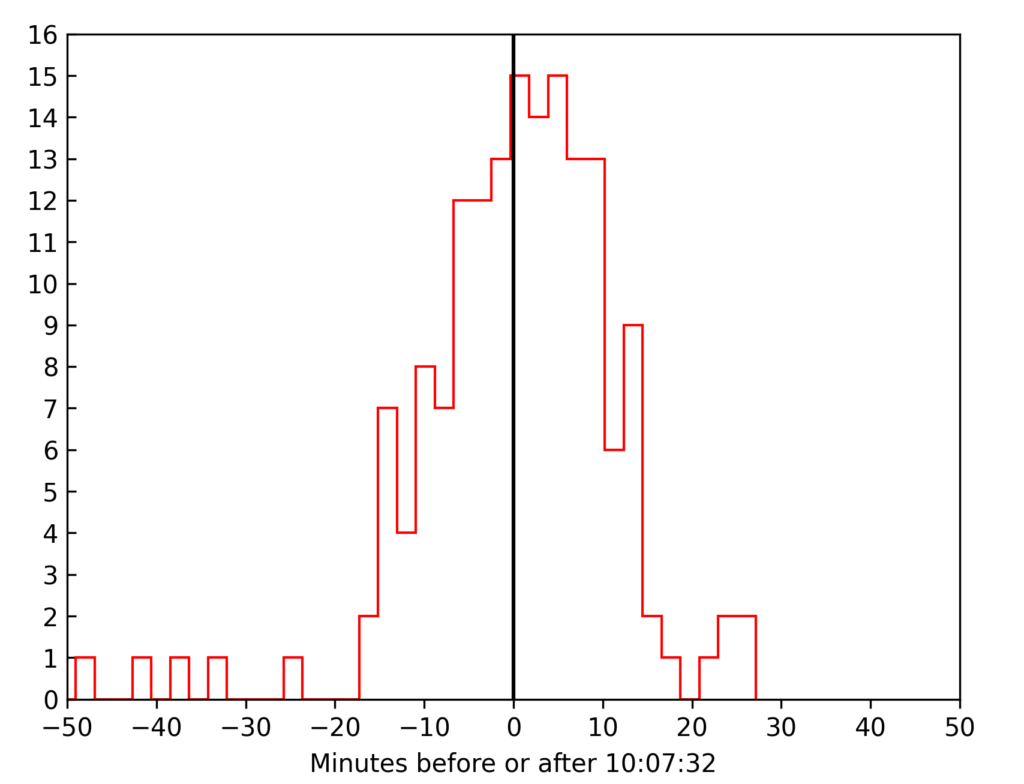
Some of you will recognize this as something that could appear like a normal distribution. In fact, we can transform the plot to make another, non-cumulative plot (if the data was truly continuous, this would correspond to differentiating the above curve), getting a histogram of the arrivals of people in certain small time intervals. This is what is shown below.

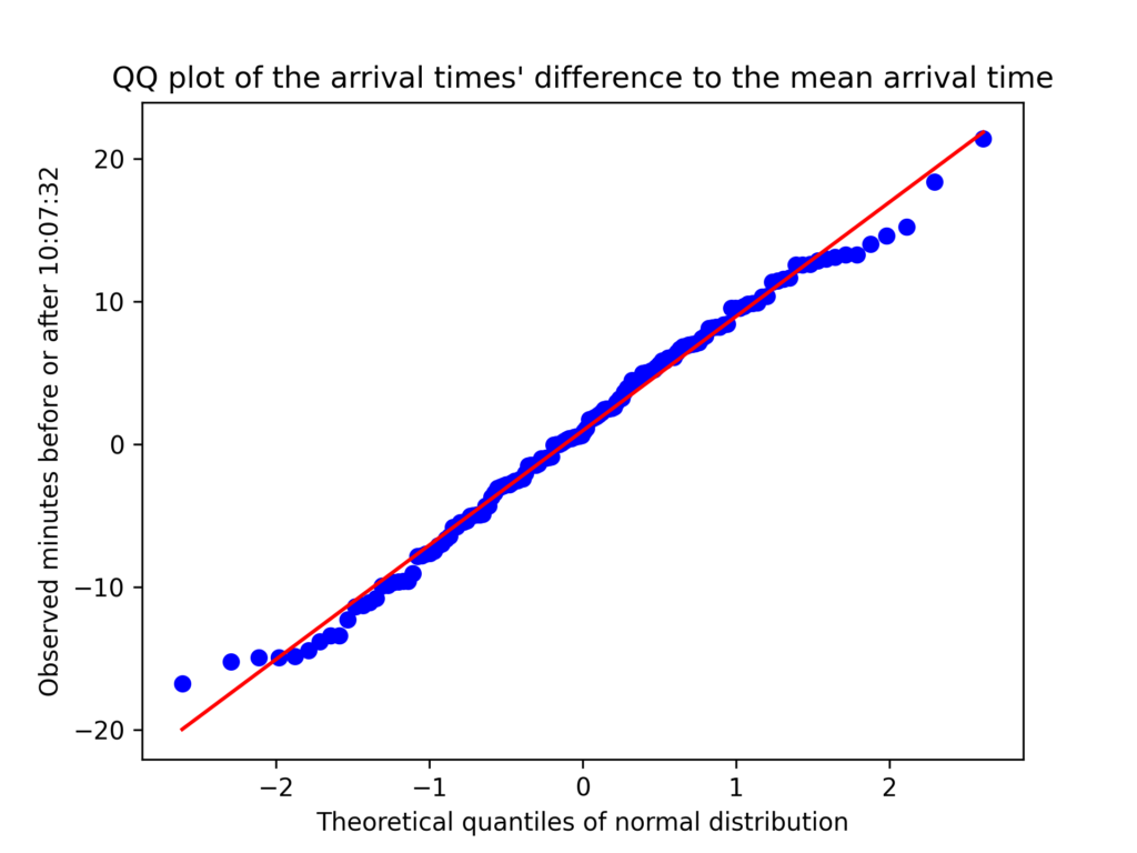
For example, we observe that 15 individuals arrived between 10:07:32 and 10:09:36 (each histogram bin has a width of 2 minutes and 4 seconds, apparently). And indeed, it does seem quite normally distributed, though curiously there are a few outliers, especially to the left (earlier arrivals). This could be partially explained by the fact that I am unsure of the arrival times of the first few people who came before I got the idea of doing this, so they are estimates, which is also apparent in the CSV file at the end of this article. Removing the first six and last four observations (although there might be some caveats with doing this, which I am unsure of), the following QQ plot shows that the arrival times could reasonably be assumed to be normally distributed.

Although we cannot know if it is normally distributed without analyzing human behavior, it does indeed “closely resemble” it. As mentioned, I initially found this slightly surprising. But then I mentioned it to a fellow Physics student who simply commented that “everything in real life is normally distributed.” Fair point, I guess. ¯\_(ツ)_/¯ Results in mathematics such as the Central Limit Theorem also have the normal distribution play a key role, so maybe it is not so surprising after all.
A closing remark is that the arrivals are neither independent nor identically distributed: People arrive in friend groups, so the arrivals are “chunked”. It is also quite likely that a given person is often early or often late. Nonetheless, it could be interesting to investigate this further and back it up with more data.
Data collection
In case you are wondering, in order to record all the arrival times without going insane, I just ran this Python script each time I saw someone enter the auditorium. There might be better ways to do it, but this worked quite well.
from datetime import datetime
import logging

logging.basicConfig(level=logging.INFO, filename="log.log")

logging.info(datetime.now().strftime("%H:%M:%S"))
I then reformatted the generated log file to a CSV file afterwards, which you can download below if you want. If you use Pandas in Python, you can load it with the following.
df = pd.read_csv("arrivals.csv", index_col=0)